Calibrating What Behavior Can Identify

What can we learn from behavior?

Watching someone choose a route tells us something about what they value. But the same route might reflect a preference for speed, safety, or comfort. Inverse reinforcement learning tries to infer these preferences as a reward function. Usually, several rewards explain the same behavior.

This paper asks when a calibrated set of reward explanations is enough to support a safe decision. Conformal calibration uses held-out behavior to choose the set’s size. We build a score that measures reward differences by their effect on policy values, then identify what is needed to turn a guarantee about behavior into a guarantee about the reward behind it.

Building on conformal prediction, IRL, and conformal inverse optimization (CIO), the contribution is a decision-based calibration score and an analysis of when its reward sets can support a policy that is no worse than a chosen baseline. CIO already uses calibration and assumes a bound on ambiguity; we adapt these to IRL and analyze the resulting guarantees and limits.

The idea in two pictures

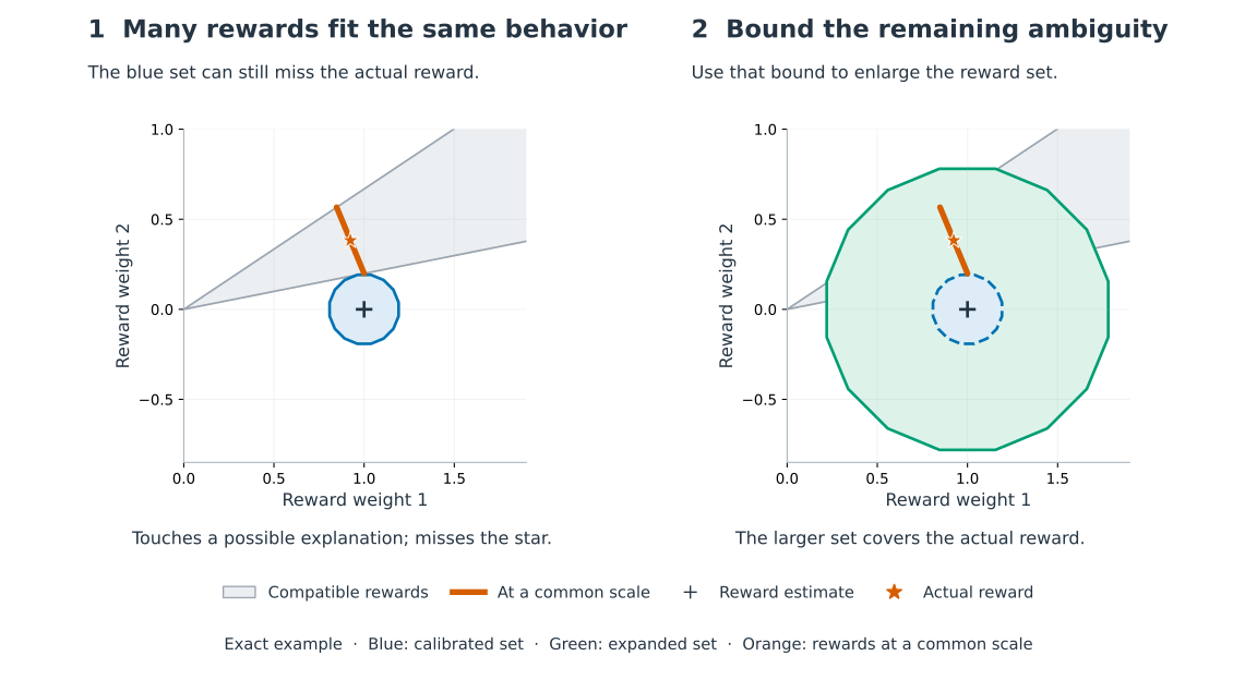
A set can contain a reward that explains someone's behavior while missing the reward they actually use. Our approach closes that gap using a bound on how different the compatible rewards can be.

Read the star first: it is the demonstrator's actual reward. Every reward in the gray region explains the same behavior. The blue set reaches that region, yet misses the star. The orange segment puts compatible rewards at a common scale so we can compare their spread. A proven bound on that spread tells us how far to expand the set; the green set now covers the star. Download PDF.

What exactly does calibration guarantee?

Under the paper's assumptions, the blue set intersects the reward set of a new demonstrator with probability at least the chosen level γ. This means it contains some reward explaining that behavior, not necessarily the demonstrator's normalized actual reward. A certified bound η on the diameter of each compatible unit-span reward set upgrades this to reward containment: R = min{2, 2q + η}, where q is the calibrated radius.

This is a marginal guarantee: the probability averages over calibration samples and a new demonstrator, rather than guaranteeing coverage for every person or every fitted set. It assumes a shared known MDP, fully observed exactly optimal policies, nonnull rewards and center, exchangeable calibration, and a valid width bound.

The drawing uses the exact 16-action example in Appendix D. Its axes are w = 2θ/(1−β); the span norm is max_j p_j^Tw. The polygonal sets are balls in this norm. The picture illustrates the coverage event; its proof comes from calibration and the width bound.

In a small exact example, the best worst-case gain over a baseline decreases as the reward set grows. At radius 1 or larger, the ball-based rule cannot certify an improvement. — **Covering more rewards makes protection easier, but improvement harder.** The baseline is a policy we could keep using. We choose a new policy by maximizing its worst-case gain over that baseline across the reward set. If the actual reward is covered, the policy is no worse than that baseline. A very large set can leave no provable improvement, so keeping the baseline is optimal. The curve shows one exact small example. Download PDF.

What does “safe” mean, and where does this rule stop helping?

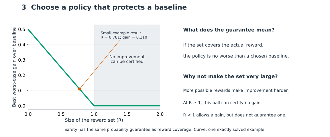
“Safe” means no worse than the reference policy in expected discounted reward. It is a comparison of policy values, not a guarantee that every trajectory avoids harm. Reward containment transfers its marginal probability of at least γ to this comparison.

For the paper's ball-shaped reward set, R ≥ 1 makes the optimal worst-case gain zero. R < 1 is necessary, but not sufficient, for a positive gain. At R > 1 all optimal policies have the same expected features as the reference; at R = 1 other policies may tie. Other reward-set shapes can behave differently.

The plotted curve is G(R) = max{0, (1−R)/2} for the 16-action example with a uniform reference. Its positive branch is example-specific. These explanatory figures were added after acceptance; see the version record and reproducible plotting source.

What the paper contributes

01 · measure the right difference

Compare what rewards do to decisions

Two coordinate descriptions of the same reward should give the same uncertainty. We measure reward differences by how much they change policy values. The resulting calibration score is invariant to feature reparameterization and can be computed by a linear program.

02 · state what is covered

A plausible explanation can miss the actual reward

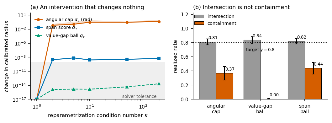
We separate two events: the set contains a reward compatible with the behavior, and it contains the normalized actual reward. At an 80% target, the original experiment observes about 82% for the first and 44% for the second.

03 · connect coverage to decisions

Show what a safety guarantee needs

A certified bound on the remaining reward ambiguity lets us enlarge the set and protect a baseline policy. We also identify when that enlargement becomes so conservative that the ball-based rule cannot certify any gain.

What the original experiments show

Original Figure 1. Left: coordinate changes move the angular radius by 0.424 radians on average at condition number 200, but the span radius by at most 2e-8. Right: score coverage is 0.812, 0.838 and 0.819 for angular, value-gap and span; containment is 0.368, 0.004 and 0.438. The value-gap score event is not set intersection despite the shared original legend. — **Left: changing coordinates should not change uncertainty.** The underlying rewards and behavior stay the same, but the angular method's radius moves by about 24° on average at condition number 200. Our span-based radius changes by at most 2×10⁻⁸. **Right: passing calibration does not imply covering the actual reward.** All three scores reach their 80% target, while actual-reward coverage is much lower.

How to read the original figure's labels and numbers

Score coverage is 0.812, 0.838 and 0.819; reward containment is 0.368, 0.004 and 0.438 for the angular, value-gap and span methods. The original figure's shared “intersection” legend means only score coverage for the value-gap baseline. The containment tests use angular, Euclidean and span geometry, respectively. The 24° result is 0.424 radians at κ = 200.

Limits of the original experiments

The original benchmarks did not demonstrate a useful certified improvement. Without a sharper bound on reward ambiguity, the safe version returns the baseline policy. It performs worse than the point estimate in all six comparisons in Table 2. A less conservative version, without reward-containment coverage, wins two of six.

The theory explains why the certified rule returns the baseline. It does not predict whether that baseline beats the point estimate. These results motivate finding tighter ambiguity bounds or using reward sets of a different shape.

Can the guarantee ever support an improvement?

Yes, in a small example where the ambiguity can be calculated exactly. We use one state and two reward features, so the compatible rewards at a common scale form a line segment. Its endpoints give a proven ambiguity bound, rather than estimating one from sampled hidden rewards.

Added after acceptance on 6 October 2026; this experiment was not part of the reviewed submission.

Appendix D: a fixed center and uniform reference, 100 independent calibration/test splits. Values are common across splits to shown precision.
Actions	Reward ambiguity η	Set size R	Worst-case gain over baseline
16	0.397825	0.780508	0.109746
4 (control)	2	2	0

With 16 actions, the expanded set still supports a provable gain of 0.109746 over the uniform baseline. Directly calibrating the farthest compatible reward gives a tighter set and a larger certified gain of 0.209202. Both methods choose the same action, so this strengthens the guarantee rather than improving the policy.

With four actions, the ball-shaped set gives no certified gain. Keeping the exact compatible reward set instead gives a gain of 0.5 in this control. This shows that the shape used to represent uncertainty can itself limit the decision.

This deliberately small example does not establish useful widths for the original benchmarks, scalability, or superiority to point-estimate IRL. It was added after acceptance and was not part of the reviewed submission.

Read Appendix D Experiment script Recorded results Version and change record

Inside the repository

envs/tabular MDP, gridworld, Objectworld

irl/LP-IRL, MaxEnt, Bayesian, Bellman feasible sets

conformal/span seminorm, score, quantile, the q → R bridge

robust/occupancy-space robust MDP solvers

cio/the upstream reference implementation

paper/dated author revision, figures, unchanged accepted submission

Repository & reproduction instructions Where each number comes from

Cite this

@inproceedings{chi2026cpirl,
  title     = {Calibrating What Behavior Can Identify:
               Conformal Reward Sets for Inverse Reinforcement Learning},
  author    = {Chi, Yuhan},
  booktitle = {Physical Understanding for Decision-Making:
               Bridging Foundation Models and Reliable Agents},
  series    = {NeurIPS 2026 Workshop},
  year      = {2026},
  note      = {Poster}
}

CITATION.cff